Formula Auditing
Trace Precedents
-
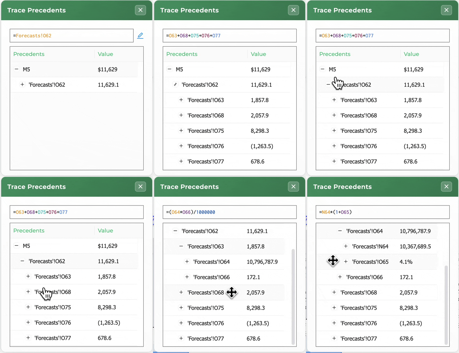
See all the cells referenced in your formula in one view
-
Quickly jump to every precedent cell using the up and down arrow keys
-
Make spreadsheet edits without having to close the trace precedents window
-
Dive a layer deeper and view the precedents of the precedents cells from the same window without having to rerun the tool
-
Close the window by hitting "Esc." Never need to touch your mouse!
-
Similar to the tracing precedents tools seen in plug-ins like Macabacus, Arixcel, Factset, and S&P Capital IQ on Excel
Trace Dependents
-
See all the cells that reference the cell that you’re on in one window
-
Navigate to every dependent cell using the up / down arrow keys
-
We've optimized the tool for speed, and if there is a time-out due to the complexity of the spreadsheet, we'll let you know and return anything that we've already found
-
If a Sheet is expected to have a timeout, we will notify you and you can then choose individual tabs to search versus the entire Sheet
-
Close the window by hitting "Esc." Never need to touch your mouse!
-
Similar to the trace dependents tools seen in plug-ins like Macabacus, Arixcel, Factset, and S&P Capital IQ

Goal Seek
-
Determine the precise input required to automatically hit any desired outcome, without manual trial and error
-
Select the Set Cell whose result you want to control. This cell must already contain a formula.
-
In To Value, enter the target result you want the Set Cell to return.
-
Select the By Changing Cell, which is the single input that will adjust to reach the target.
-
Optionally, adjust tolerance and maximum iterations to control how precisely and how long Excel searches for a solution.
-
SheetWhiz will then calculate and return the Goal Seek result, updating the changing cell accordingly.
What If Analysis
-
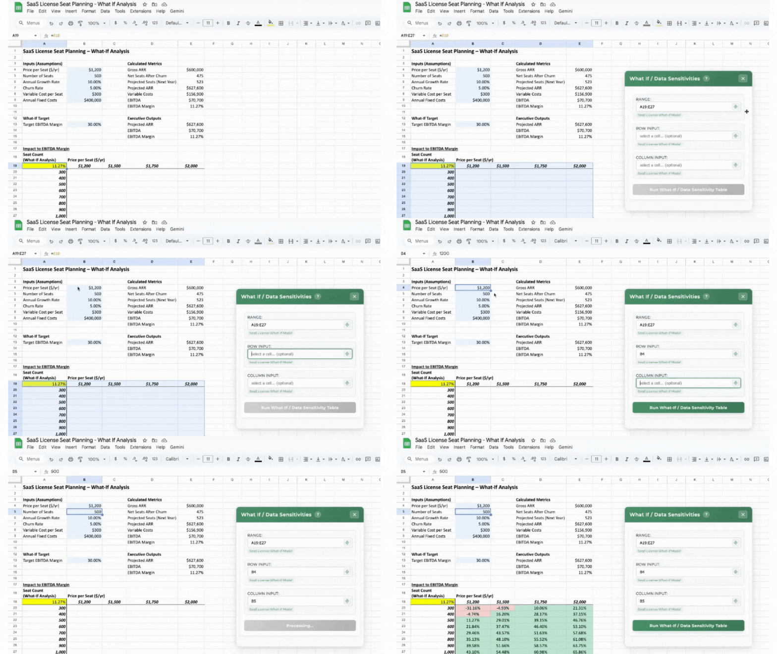
Build Excel-style financial models directly in Google Sheets by instantly testing how changes to key inputs impact outputs like revenue, profit, or margin, without duplicating sheets or rewriting formulas.
-
Start by selecting the outcome you want to model. This must be a formula cell, such as total revenue, EBITDA, or cash flow, just like in Excel financial modeling.
-
Define the range of input values you want to test and select the full modeling range, including the end-result formula cell, to create a What-If Analysis data table in Google Sheets.
-
Assign Row Input and Column Input cells to one or two variables, such as price, volume, or costs, so SheetWhiz can automatically substitute values and recalculate results at scale.
-
Run What-If Analysis to compare best-case, worst-case, and expected scenarios, or pair Goal Seek to calculate the exact input required to hit a target outcome, bringing Excel-style modeling workflows to Google Sheets.

Format Cycles
General Number Cycle
-
Apply custom number formats to selected cells quickly
-
Use our shortcut once, and "Format 1" will be applied to the selection. Use our shortcut again while still on the same selection, and "Format 2" will be applied. Use it again and "Format 3" will be applied. There are 4 formats that you can cycle through
-
All formats are completely customizable, meaning you'll be able to apply any format you want to your selection quickly and without a mouse
-
Some users would like multiple cycles because they want cycles specific to percentages, multiples, currencies, etc. We provide cycles for all of these number types (i.e., General Number Cycle - 6 Formats, Percent Cycle, Indentation Cycle, Date Cycle, Local Currency Cycle, Foreign Currency Cycle, Multiples Cycle, K, M, bps, SOFR Cycle) and they work the same way as General Number Cycle

Font Color Cycle
-
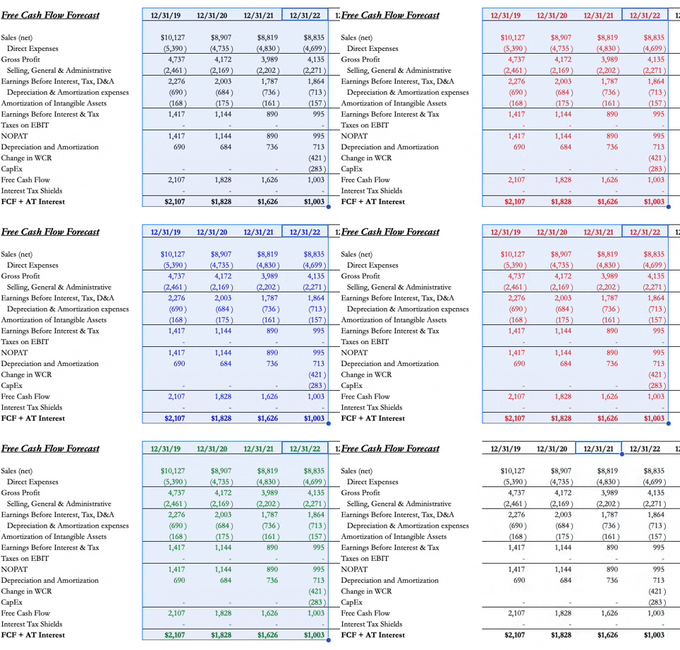
Apply font colors to selected data
-
Most users use this to quickly color-code different data types in their sheet
-
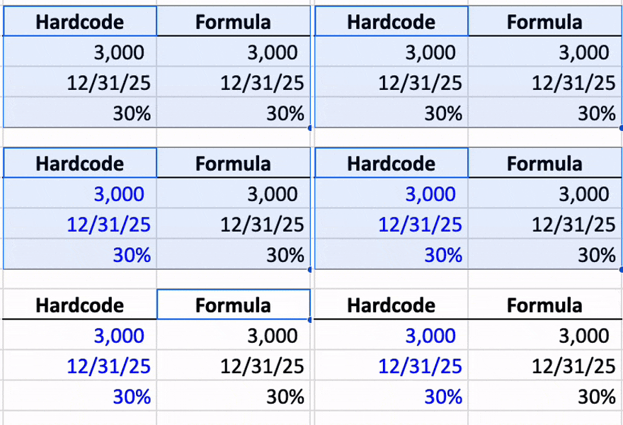
Blue = Hardcode
-
Green = Formula uses an input from another tab
-
Red = A one-off formula adjustment or an error to return back to
-
Black = Formula
-
-
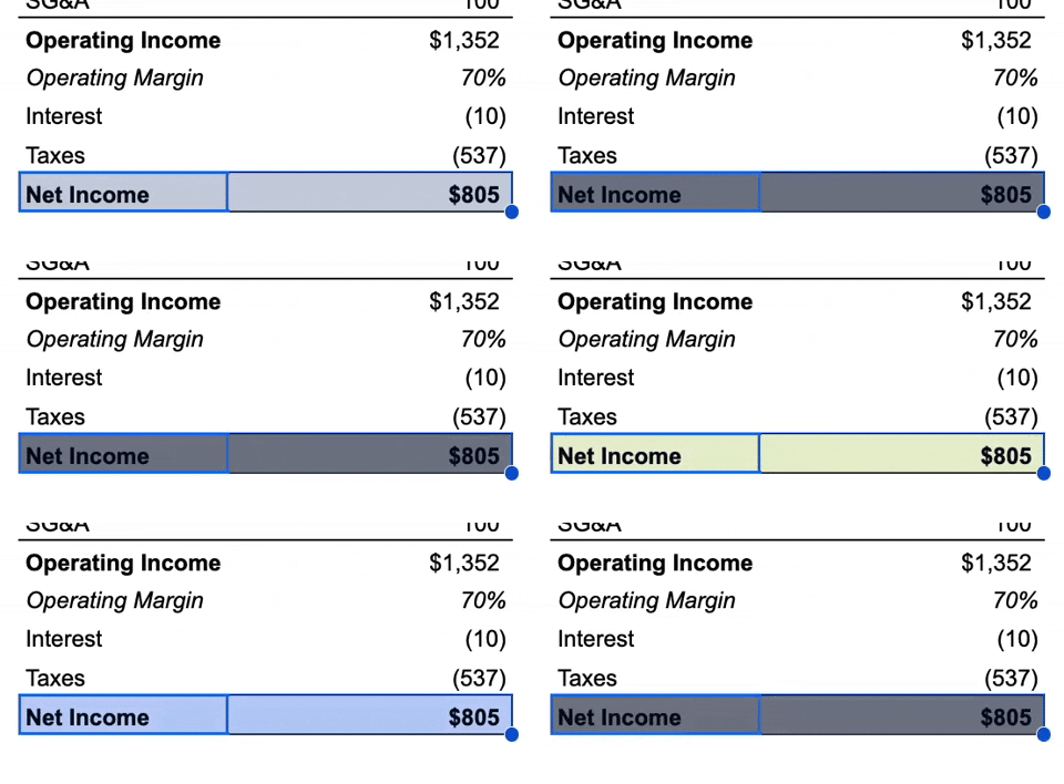
Use our shortcut once, and "Color 1" will be applied to the selection. Use our shortcut again while still on the same selection, and "Color 2" will be applied. Use it again and "Color 3" will be applied. There are 4 formats that you can cycle through
-
All colors are completely customizable, meaning you'll be able to apply any format you want to your selection quickly and without a mouse
Fill Color Cycle
-
Apply fill colors to selected cells
-
Most users use this to apply company colors to their analysis
-
Use our shortcut once, and "Color 1" will be applied to the selection. Use our shortcut again while still on the same selection, and "Color 2" will be applied. Use it again and "Color 3" will be applied. There are 4 formats that you can cycle through
-
All colors are completely customizable, meaning you'll be able to apply any format you want to your selection quickly and without a mouse
Auto-Color
Auto Color Selection or Sheet
-
Identify and then color cells that have hardcoded values or link to another tab
-
Hardcoded values mean any cells that has only a numerical value in the cell without an "=" sign. For example, =5 would not be a "hardcoded value" but 5 would be
-
Hardcoded values include cells that are formatted as non-numbers such as dates (12/31/24 will be a hardcoded value)
-
Linked cells are cells that reference a cell on another tab
-
Note: Once auto-color has ran, you CANNOT UNDO the changes
-
Auto-color the entire tab by using "Auto-Color Sheet" instead of "Auto-Color Selection"
-
Auto-Color Sheet: Ctrl + Shift + A
-
Auto-Color Selection: Ctrl + Shift + S
-
Export Selection as Image
Export Selection as Image
-
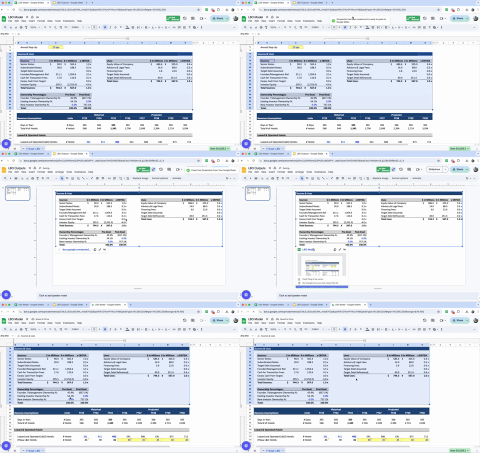
Export your selected cells as an image that you can paste to Google Slides or Google Docs so you are never screenshotting again
-
Get the exact selection you want versus approximating the output with a screenshot
-
Select the cells, hit "Ctrl + Shift + C" or trigger the shortcut via the Paste Special menu
-
Once you are notified that the image is ready to paste, go to where you want to paste the image and paste the image as you normally would
-
The pasted image will have a link to the cells that were screenshot
-
Note, for higher quality images, zoom in on your selection. The bigger the selection is on your screen, the higher quality the image
-
Ability to update images automatically is a work in progress!
Excel Shortcuts on Google Sheets
We support the following Excel shortcuts
-
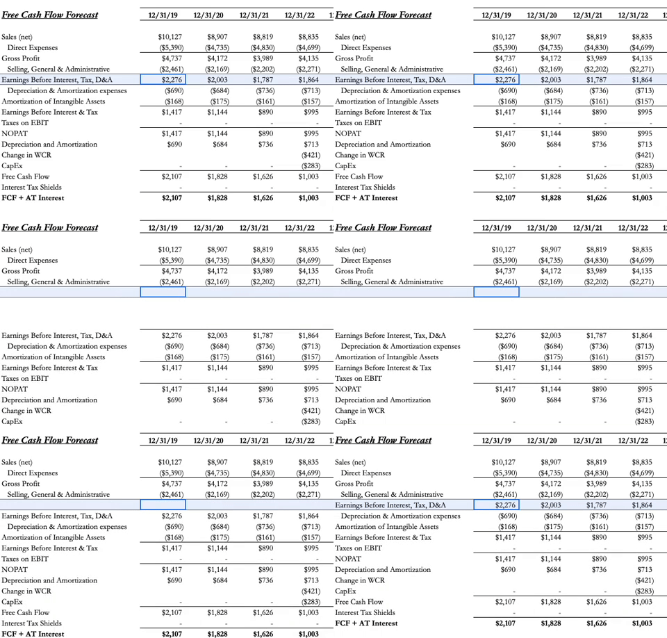
Insert Columns / Rows: Ctrl + Shift + "+"
-
Delete Columns / Rows: Ctrl + Shift + "-"
-
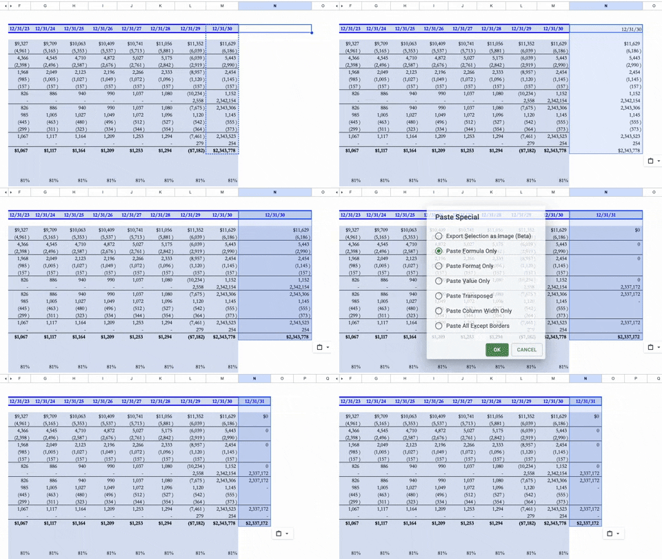
Paste Special: Alt/Option + E + S . This will bring up a menu with the following options
-
Export Selection as Image (Beta): Alt/Option + E + S + S
-
Formulas: Alt/Option + E + S + F
-
Values: Alt/Option + E + S + V
-
Formatting: Alt/Option + E + S + T
-
Transposed: Alt/Option + E + S + E
-
Column Width Only: Alt/Option + E + S + W
-
All Except Borders: Alt/Option + E + S + X
-
-
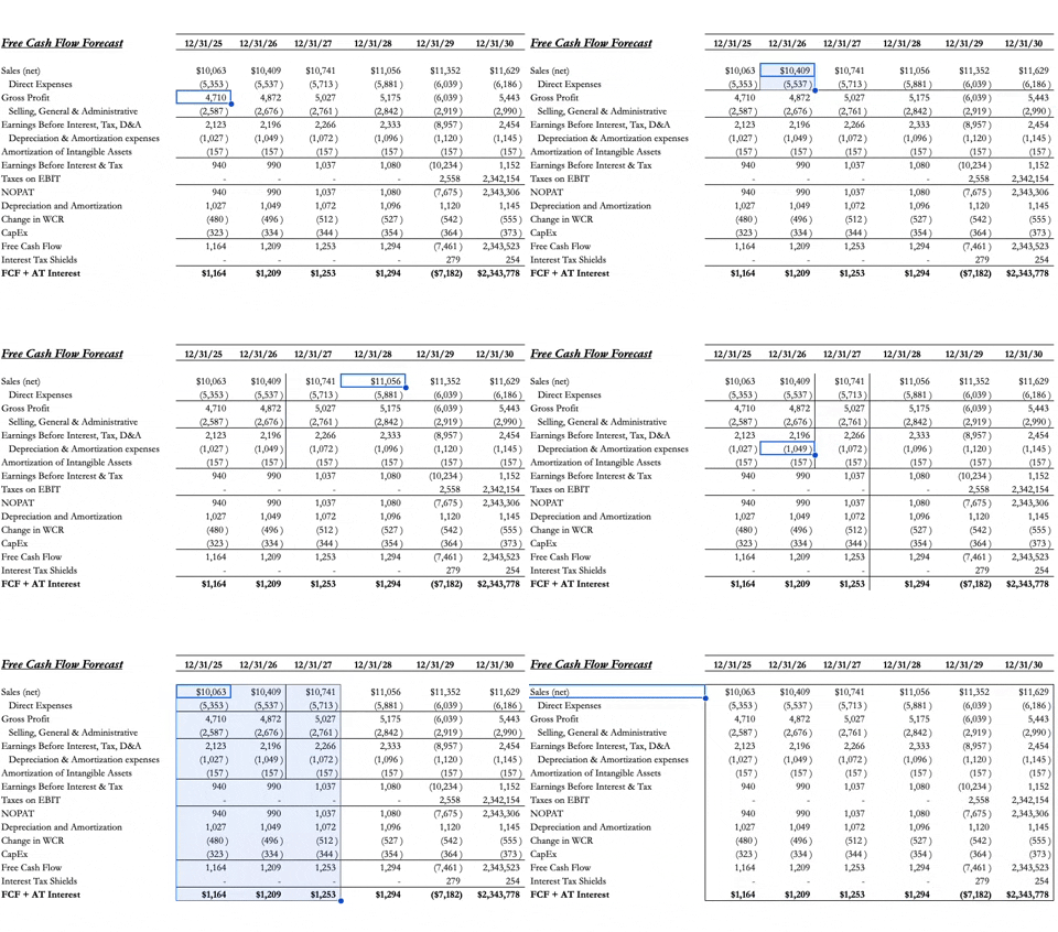
All Border Shortcuts
-
Top Border: Alt/Option + H + B + P
-
Bottom Border: Alt/Option + H + B + O
-
Left Border: Alt/Option + H + B + L
-
Right Border: Alt/Option + H + B + R
-
Outside Border: Alt/Option + H + B + S
-
All Border: Alt/Option + H + B + A
-
Inner Border: Alt/Option + H + B + I
-
Horizontal Border: Alt/Option + H + B + Z
-
Vertical Border: Alt/Option + H + B + V
-
Remove Border: Alt/Option + H + B + N
-
-
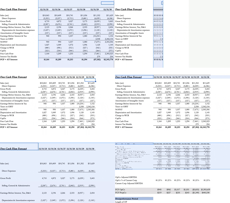
Resize Rows & Columns
-
Set Column Width: Alt/Option + H + O + W
-
Autofit Columns: Alt/Option + H + O + I
-
Set Row Height: Alt/Option + H + O + H
-
Autofit Rows: Alt/Option + H + O + A
-
-
Alignment
-
Align Center: Alt/Option + H + A + C
-
Align Left: Alt/Option + H + A + L
-
Align Right: Alt/Option + H + A + R
-
Align Top: Alt/Option + H + A + T
-
Align Middle: Alt/Option + H + A + M
-
Align Bottom: Alt/Option + H + A + B
-

-
Increase Decimals: Alt/Option + H + 0
-
Reduce Decimals: Alt/Option + H + 9

-
Add/Remove Filters: Ctrl + Shift + L

-
Add/Remove Gridlines: Alt/Option + W + V + G
-
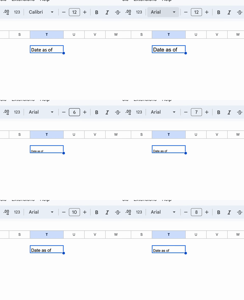
Font Shortcuts:
-
Set Font: Alt/Option + H + F + F
-
Set Font Size: Alt/Option + H + F + S
-
Increase Font Size: Alt/Option + H + F + G
-
Decrease Font Size: Alt/Option + H + F + K
-
-
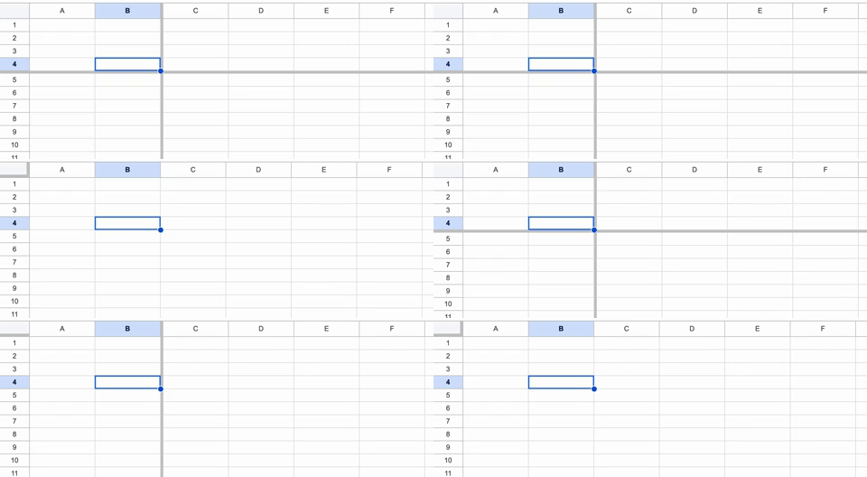
Freeze & Unfreeze Rows & Columns:
-
Freeze Columns & Rows: Alt/Option + W + F + F
-
Unfreeze Columns & Rows: Alt/Option + W + F + U
-
Freeze Columns: Alt/Option + F + C
-
Unfreeze Columns: Alt/Option + W + F + C
-
Freeze Rows: Alt/Option + F + R
-
Unfreeze Rows: Alt/Option + W + F + R
-
-
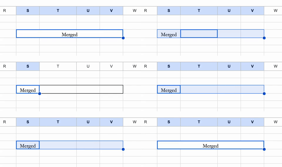
Merge & Unmerge Cells:
-
Merge All: Alt/Option + H + M + A
-
Unmerge All: Alt/Option + H + M + U
-
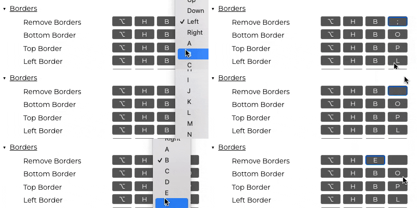
Customizable Shortcuts
All shortcuts are customizable. If you prefer a shortcut instead of the one shown as the default, you may change it by clicking the key you'd like to change
